Machine Learning for Multifactor Stock Selection

Project Overview: This project is part of an exploratory research during my internship at one securities company in China. The final conclusion is that, combining models of different configurations enhances the performance. For ethical considerations, I will not go into great details. Instead I am going to briefly decribe the task and list several empirical findings that I personally think are quite interesting. This project is mostly done by myself and this article only represents my personal point of view.

1. Task

I was given a set of stock factors that were proved to be efficient in China A-share market. My task was to explore whether machine learning algorithms could incorprate all these factors into stock selection in a way that constantly outperformed conventional methods. It was basically a multifactor stock selection problem that employed machine learning to add a flavor of non-linearity.

2. Approach

2.1 Basic framework

The stock selection was performed on a walk-forward basis. At each rebalance date, a new machine learning model was trained to incorporate the latest data. The model was then used to score the entire universe of stocks, and the top ranked stocks and their corresponding weights were saved. Finally, the stocks and weights were fed into a portfolio backtesting program.

We can also think of the time-series of scores as a composite factor originated from multiple stock factors, and test its efficiency by sorting stocks into different groups and perform the backtesting separately.

2.2 Machine Learning configurations

• Learning algorithm: I used LightGBM as the library for boosted trees algorithm. I also used vanilla feed-forward neural networks and neural networks with LSTM layers. I implemented the neural networks in PyTorch.
• Learning objective: The most typical learning objectives are regression and classification. Both fit into my task and are also supported by all three algorithms. LightGBM also supports “learning to rank”, which LambdaRank uses the normalized discounted cumulative gain as the loss function instead of the negative log likelihood and mean square error, and is typically applied in information retrieval.
• Labeling: the labelling scheme I chose depended on the learning objective. For a regression task, the label for a stock was its future return. For a classification task, typically the best-performed and worst performed stocks were labeled as positive and negative, and the stocks in between were omitted to increase the signal-to-noise ratio. For a ranking task, stocks were first sorted by their future returns and then divided into several groups.
• Dataset: The dataset as the input to the learning algorithm was the features(stock factors) data aligned with the label data. Features were available daily, but there was a resampling involved. For example, if when labeling the future return used was five-day return, then the data were included every five days. Regarding the choice of dataset, I identified two factors that had material impact on the outcome. The first was the length of time window, or the periods of historical data. While a longer window guaranteed sufficient training data and reduced overfitting, a shorter window enabled the model to better respond to potential market regime shift. The second was the subsample used, which was more relevant to classification tasks. To illustrate, we can keep the top 20% and the bottom 20% performed stocks each day. We can also keep the top 20% performed stocks and randomly select another 20% of stocks.
• Training and validating: When training, a validation set was used for performance evaluation, as well as hyperparameters tuning when necessary. While hyperparameter does matter a lot, in my project it was not the main focus unless I found the loss in validation set barely declined.

2.3 Benchmark:

• The advantage of machine learning lies in its nonlinear decision boundaries. Its contrast is of course the conventional linear method. I thus used the most simple linear regression with the same set of stock factors as regressors. All else equal, I used the linear model instead of machine learning algorithms to repeat the train-validation-predict process, and used the corresponding backtest performance as a benchmark.
• There is no need to introduce regularization because the factors I was given were filtered in an effort to minimize the correlation between each other (Ridge excluded), and all of them had been proved to be effective methods (Lasso excluded). Actually adding regularization did not improve the predictive power of the linear model that much.
• That being said, the backtesting module used several major equity indexes as benchmark.

2.4 Ensemble model

As we can see in the Machine Learnig configurations section, there are so many alternative choices. In fact, in my test, I failed to find such thing as the most perfect configuration. Some were better as with absolute return, others exhibited lower volatility and drawdown. This reminded me of Ensemble Learning, a machine learnig paradigm aggregating a group of weak learners to achive a better predictive performance. During my internship, I figured out a way to combine the results from models varying in the learning algorithm, objective and datasets, which obtained a better predictive performance and backtesting outcomes than any configuration alone. In this report, the results I present was achieved by fixing classification as the default learning objective and altering algorithms and datasets(different time windows/subsamples). The algorithms I chose include LightGBM(LGB), vanilla feed-forward neural networks (ANN) and networks with LSTM layers(LSTM). I used two time windows, namely 2 years and 1 year, denoted as 100 and 50 respectively because they coresponded to data from 100 and 50 trading days. I labeled the data in three ways which corresponded to three subsamples: 1) label top 20% stocks as postive and bottom 20% as negative(TB); 2) top 20% as postive and randomly selected 20% as negative(TR); 3) bottom 20% as negative and randomly selected 20% as postive(RB). Taken together, I set up 3 x 2 x 3 = 18 different configurations.

3. Findings

• Models with different configurations are far from perfectly correlated.

In particular, the predicted scores of TR models are negatively correlated with TB and RB models. Models that differ in the underlying algorithm also have limited correlation ranging from 0.5 to 0.8. This fact to some extent is favorable to the use of ensemble paradigm because the low variance of ensemble learning relies on limited correlation between constituent weak learners.

• Choice of training sets has a significant impact on the outcome.

The figures below present the results of factor backtest when different subsamples are used. Here the “factor” comes from the time series of ML-predicted scores: by using a bunch of stock factors as features for machine learning, we are basically converting multiple factors into one single factor. Stocks are sorted by this factor into 10 groups on a regular basis and portfolio backtests are conducted in each group. In each figure, the upper part presents the equity curves of ten portfolios, and the lower part presents the annualized returns of each portfolio.

The TB model, which uses the data of stocks with the top 20% and bottom 20% performance cross-sectionally, has the best performance in the magnitude of long and short returns. It is not surprsing, because this way of using data results in relatively high signal-to-noise ratio, and is somewhat the default setting practioners use. The test on RB model shows that the short portfolio (the 10-th group) has -38.69% yearly return, which is impressive. What’s more, the monotonicity of ten portfolios are excellent. TR model does not give a equally good performance, but the monotonicity of ten portfolio still holds with few exceptions. What is surprisinig is that, when combining the factors from TR and RB into one, the backtesting outcome is very similar to TB model alone. This is a strong evidence that aggregating models of different configurations tend to enhance the performance.

Figure 1 TB—long return: 46%, short return: -43.56%

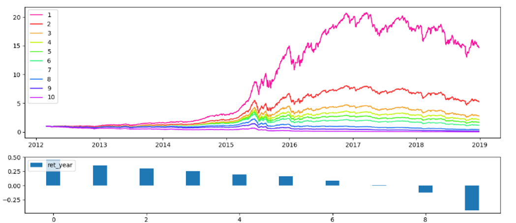
Figure 2 TR—long return: 26.20%, short return: 7.06%

Figure 3 RB-long return 36.44, short return: -38.69%

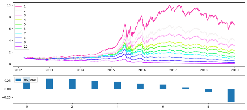
Figure 4 Combininig TR with RB—long return: 46.51%, short return: -34.11%

Not only does choice of subsample make a difference, the length of time window also matters. Table 1 reports the results of the portfolio test where the 100 stocks with highest scores were selected at each portfolio rebalance date. Section 2.4 points out that I tested 18 models of distinct configurations, differing in algorithms, subsample or time window. XXX_Composite thus corresponds to combining the scores of models with XXX configuration into one composite score and select stocks accordingly. While I am going to analyze the table again later, here we focus on the results for 100_composite and 50_composite. As I expected, using data from less trading days can make the model more sensitive to the change of market style, thus reducing the max drawdown which usually happens when the market regime shifts. Also, using more data tend to train a more robust model that works better, especially in stable market condition which is usually the case. Consequently, 100_composite still defeats 50_composite in annualized return despite a larger max drawdown.

• The composite model is the best one.

As is shown in table 1 below, the composite model that aggregates 18 models achieves the best annualized return, and are ranked the 2nd in other metrics except the turnover ratio.

Table 1 Performance metircs of different models 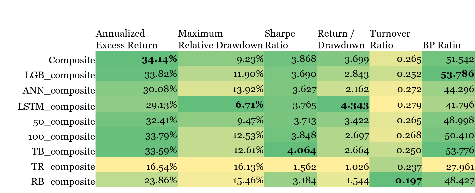Note: Maximum Relative Drawdown uses CSI 500 index as the benchmark

It is not surprising that the composite model has the best return performance, because all the labels are generated only taking future return into consideration. I believe that, if when labeling, we use the future return divided by stock volatility as the sorting criteria, which is esentially analogous to sharpe ratio , then the composite model will achieve the best sharpe ratio, probably the max relative drawdown at the same time. This argument leaves open the possiblity of addding another variation of the model configuration to further enhance the performance.

Finally, figure 5 shows the equity curve corresponding to the portfolio test of the composite model. The red line is the relative equity curve benchmarked against CSI 500, which is upward most of the time but goes down a little bit during 2017, a year when China A-share Market experienced a major regime shift. The drawdown, however, should be more of a problem to the set of factors I use.

Figure 5 Backtest equity curve: the composite model Note: Black: portfolio equity curve; green: CSI 500 index equity curve; red: portfolio equity curve relative to CSI 500